Last updated on Saturday, October 17, 2026

Week 6: Parallelism

Congrats on completing your sixth week of CS-214! Here is a round-up of interesting questions, tips for exercises and labs, and general notes about the course.

Administrivia

• Break: enjoy the autumn break next week! There won’t be any lectures, nor will be there by any labs due.

Interesting Ed questions

• Could perfect specs and tests remove the need to review AI-written code?

Exploring the limits of parallelism

How many servers should you buy for your start-up?

During lectures we studied the notions of work and depth. They describe the total number of computational steps, and the minimum number of computational steps if we had unbounded parallelism, respectively. Let’s explore the case when we have bounded parallelism, i.e. a limited amount of resources.

Recall the definitions of work and depth:

• $W(e_1 ; e_2) = W(e_1) + W(e_2)$

• $W(parallel(e_1, e_2)) = W(e_1) + W(e_2)$

• $D(e_1 ; e_2) = D(e_1) + D(e_2)$

• $D(parallel(e_1, e_2)) = max(D(e_1), D(e_2))$

where $e_1; e_2$ denotes two expressions that run in sequence.

By analysing a program, like segmentPar from the lecture slides, we can compute the asymptotic complexity (depth) $D$ if we had infinite parallelism.

Amdahl’s law

Amdahl’s law describes the speed-up we can achieve in a program, given an amount of parallelism $P$. It assumes that a fraction $p$ of the work $W$ in the program is parallelisable and a fraction $1-p$ is sequential. For a given amount of parallelism $P$ (e.g. the number of cores, or threads), we can compute the run time of the program: $$t = (1-p)W + \frac{pW}{P}$$

If we plug in $P = 1$ (no parallelism), we obtain that $t$ is simply the total amount of work $W$. If we plug in $P \rightarrow \infty$, we obtain that $t$ is merely the sequential part of our program $(1-p)W$, which is $D$. Rewriting the formula for the case $P \rightarrow \infty$, we can determine the parallelisable fraction $p$ if we know the depth $D$: $$p = 1 - \frac{D}{W}$$

Business economics 101

Armed with the ability to compute how much we gain from increasing resourcing, we can now find the optimal amount of resourcing to source for our start-up! (Or our GPU machine learning research project).

Let’s assume for simplicity that the success $S$ of our venture (e.g. profit, cyber threats detected, vaccines produced, Kaggle score) scales linearly with our program throughput $T = 1/t$: $$S = k * T = \frac{k}{t}$$

Additionally, our cloud provider, or server vendor, provides us with a cost formula per core: $C = P$. Only €1 per core! Subtracting the resource cost $C$ from the success $S$ gives us the net success: $N = S - C$.

Let’s analyse our net success for different amounts of parallelism, and for different parallelisation fractions.

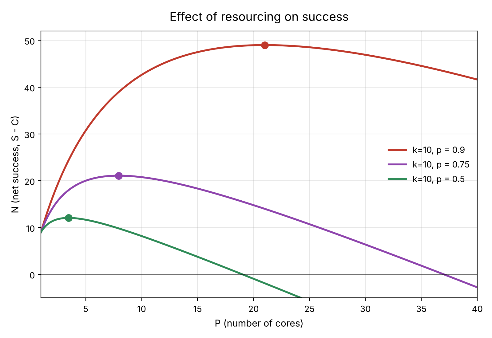
We benefit from investing in more resourcing (parallelism), but only to a certain extent. Beyond some point we pay more for extra resourcing than we gain from throughput. However, as we make programs more parallelisable, it pays to invest in more resourcing!

Range: What does i <- 1 to n mean in for-expressions?

Scala provides a nice way to iterate over a range of values:

def printToOneThousand = 
  for i <- 1 to 1000
  do println(i)

But what does 1 to 1000 actually mean? This is the same as writing 1.to(1000) (documentation), which creates a sequence of numbers (of type Range).

The following functions are equivalent to our example:

def printToOneThousand =
  for i <- Range.inclusive(1,1000)
  do println(i)

def printToOneThousand = 
  Range.inclusive(1,1000).foreach(println)

The expression 1 to n is a shorthand for a range from 1 to n, which includes n. To create a range that excludes n (i.e. stops at n-1), you can use until instead.

Ranges offer more than just this! It’s possible to create a Range over characters, or even with different step sizes:

for
  i <- 1 until 5 // Seq(1,2,3,4)
  j <- 'a' to 'd' // Seq(a,b,c,d)
  k <- 1 to 10 by 5 // Seq(1,6)
do
  println(s"i = $i, j = $j, k = $k")

Code quality improvements

Here are a few common code smells and code style improvements, based on your lab submissions:

More combinators

Thinking of a solution as a recursive function written from scratch is a great way to start and gain intuition, but as we saw in the week 3 exercises, it can be made more concise using folds, or other methods (also see week 4 debrief):

Before:

def subsets(set: MultiSet[A]): List[MultiSet[A]] = set match
  case Nil => List(Nil)
  case (item, count) :: xs =>
    val tailSubsets = subsets(xs)
    tailSubsets ++ (for
      subset <- tailSubsets
      n <- 1 to count
    yield (item, n) :: subset)

After:

def subsets(set: MultiSet[A]): List[MultiSet[A]] =
  set.foldRight(List(List.empty)) { (e, acc) =>
    acc ++ (for
      subset <- acc
      n <- 1 to e._2
    yield (e._1, n) :: subset)
  }

Or when aggregating data, groupBy can be much more concise than foldLeft:

Before:

val counts: Map[A, Int] =
  seq.foldLeft(Map.empty) { (m, x) =>
    m.updated(x, m.getOrElse(x, 0) + 1)
  }

After:

val counts: Map[A, Int] = seq
  .groupBy(identity) // Use the value directly for equality tests, yields Map[A, Seq[A]]
  .map((v, occurrences) => (v, occurrences.length)) // The length of the Seq[A] is what we needed

This is also a common pattern in many computing problems, especially when parallelism is involved (see MapReduce on Wikipedia and groupMapReduce in Scala).

Better comprehensions: Avoid redundant .toList

Instead of using a redundant .toList, use the first generator in the comprehension to force the output type to a List:

Before:

(for
  a <- 0 to count
  b <- someList
yield f(a, b)).toList

After:

for
  a <- (0 to count).toList
  b <- someList
yield f(a, b)

Better comprehensions: Use to for inclusive ranges

Prefer using to instead of until when using inclusive ranges:

Before:

k <- 0 until (count + 1)

After:

k <- 0 to count

Performance costs

In general, you should be aware of the performance cost of the code you write. See this summary.

For example, repeatedly using List.find can get costly, especially when the list is large. In many cases, creating a Map is advantageous, which usually has cost $O(n)$ and is only done once, and allows you to query any value in constant time, while find is $O(n)$ and will be called many times.

Before:

listA.map { (a, b) =>
  listB.find(x => x._1 == a) match
    case None    => ???
    case Some(v) => ???
}

After:

val listBMap = listB.toMap
listA.map { (a, b) =>
  listBMap.get(a) match
    case None    => ???
    case Some(v) => ???
}

Appends (:+) also have a high cost with standard Lists, but there might be ways to rewrite the code to perform better, for example:

Before:

def duplicate(list: List[A]): List[A] =
  def loop(rem: List[A], acc: List[A]): List[A] = rem match
    case Nil => acc
    case x :: xs => loop(xs, acc :+ x :+ x) // O(n) append to preserve order

  loop(list, Nil)

After:

def duplicate(list: List[A]): List[A] =
  list.foldRight(List.empty[A]) { (x, acc) =>
    x :: x :: acc // O(1) prepend, order preserved naturally
  }

“When you have a hammer…”

Here the first for comprehension is redundant and can be absorbed into the second:

Before:

val first = (for k <- 1 to n yield (x, k)).toList
for k <- first; l <- second yield (k, l)

After:

for k <- 1 to n; l <- second yield ((x, k), l)

Of course here the work done by the first one is very small, and more complex code would benefit from the separation.

For something like a simple transformation, it might be better to simply use map:

Before:

val b = for x <- a yield someFunction(x)

After:

val b = a.map(someFunction)

© 2023–2026 EPFL. CC BY 4.0.